Module 10: Homeland Security - Protect

Module 10 is the final module in the Applications for GIS class before the Final Project. It is a continuation of the previous week's work which was preparing Homeland Security layers for a simulated threat to North America Aerospace Defense Command (NORAD). Last week all the layers were prepared and this week analyses was done based on those layers.

Three of the maps from this weeks module are posted here. I'm at a loss for anything to say about these other then that I was very confused throughout the exercise by many of the instructions that seemed fairly reasonable but did not seem to work correctly and may be because the previous weeks data was not prepared correctly due differences in the previous weeks instructions and things that needed to be done such as repairing data sources and re-projecting layers.

Unfortunately, at this point I've invested way too much time in the lab to start from scratch and am posting the items that were completed as best I could.



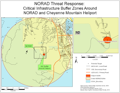
The first map shows a 500 foot buffer around a heliport that is within the initial 3-mile buffer around the entrance to NORAD that was created to identify critical infrastructure that may be involved in secondary threats in the event of a threat targeting NORAD itself. None of the steps was difficult but when I selected GNIS points to get critical infrastructure within the buffer, only 49 sites were selected (not 50). However, the one outlier site was right along the border so I just selected it and continued on. I did have the exact mix of sites by Feature Class.However, I think there might e an issue with my projections though I'm not sure what it is and why it's occurring. I seem to be getting datum conflicts when running the various Arctools. They don't stop the tool from processing though but are just warnings.



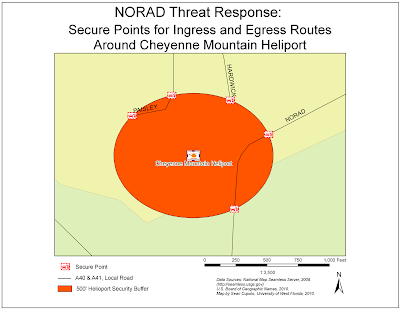
The next map is a blow up of the buffer around the heliport where ingress and egress points were identified for the roads leading to the heliport. These roads will need to be secured in the event of an actual threat so locating where to set up the checkpoints to secure them is the purpose of the map. I like the symbols that I found for these points. They were in the ERS Homeland Security set. Again, nothing was difficult about creating the map, but I think the distances may be slightly off.

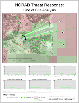
The last map shows a line of site analysis for points around the entrance to NORAD. The purpose of the map is to provide site line information to enable the placement of monitoring locations and surveillance cameras to allow all areas around and leading into NORAD to be properly surveyed for threats.



I had the most difficulty getting this map together. First there was problems creating a hillside shading raster from the initial DEM file provided. I had to take the file provided this week, follow last weeks exercise to re-project it and then I could get the hillshade to look the way I believe it should. At that point the exercise in generating a viewshed gave all kinds of problems. First we had to create surveillance points based on a description in the lab as to where to put them that did not give a good idea where they needed to go or how many to place. Inti ally I placed some on the entrance road. When I ran my viewshed, it showed all areas as visible. so I re-edited my points and tried again. Note that running the viewshed analysis at that time took at least twenty minutes a go. I thought maybe created my Hillshade file incorrectly, but am not sure because the lab does not tell you to use this file, it says use the DEM layer. However, that layer seemed to give me worse results (about half the DEM layer was green), So finally, I recreated the hillshade layer and set my points at only 2 and was able to get non-visible areas. Problems were encountered with the 3D Analyst Line of Site tool because the tool was defaulted on the DEM layer and so each line of site that was set was not reading off the correct layer to plot a line of site profile graph. When I realized that, I was able to complete the map as shown. Again, however, moving on and trying to complete the final step which was to show the line of site in ArcScene, failed completely as my lines of site show way too far from the Orthoimage of NORAD to make sense.

Module 8 Law Enforcemet: Washington DC

The posted maps where completed for the Week 8 activity if the University of West Florida On-Line GIS Certification program class, Applications in GIS (GIS4048). The focus of the week was Law Enforcement and GIS and the goal of the activity was to use GIS to analyze crime and police station data and make recommendations based on the data for adjustments to current patrols.

Maps are being posted now. Background to follow:


The first map is a base map of Washington DC showing the location of police stations and crime incidents that occurred in August 2009.


The next map shows crime proximity to the police stations. The proximity color bands were created using a Multiple Ring Buffer tool to measure proximity at intervals of 0.5, 1.0 and 2.0 Miles from each station.


The third map shows Crime Densities for three specific types of crime: Burglary, Sex Abuse and Homicide. The densities were created using a GIS Spatial Analysis tool called, Kernel Density.


The final map also uses the Kernel Density tool to show a time series snap-shot of auto theft crimes based on when they occur in a 24-hour day.

The biggest issue I had in developing these maps was the slow refresh rate of the computer. For some reason, every adjutment to a map I made required long refresh times. I tried to use the Map Cache toolbar to alleviate the re-draws but it did not seem to be working for me. The lab also included some time savers like saving a Base Map to use over and over again. Unfortunately, I failed to get my basemap set correctly at the beginning based on the later labs so I still ended up with a lot of redo work which was particularly painful in regards to trying to get the road labels to diplay correctly. I did figure out a useful trick though on the fourth map which was that it was just as easy to compy the first data frame with all it's layers in it to three additional layers (then the Frame Properties were already set). I also found it easier to compose the map before adding everything. Finally, I had major problems using the graphing tool on this lab such that I decide it was more effective to export data from the graph tool to an Excel spreadsheet and create the graph there then copy it back to the map. The last two graphs were done using these procedures and they look much better then the first one.