Finale Project - Manatee-Bobwhite Transmission Line

Here are the submissions for the final project.

Presentation

Written Summary

The posted maps were completed for the Week 11 Lab for the University of West Florida Online GIS Certification program class, Introduction to Geographic Information Systems (GIS 4043/L). The maps was created using the ArcGIS ArcMap program and based on data from ESRI Virtual Campus courses.

Creating and Editing Labels and Annotation

I was planning on taking this ESRI course anyway so doing it for class worked out well. I'm going to go back and do the Annotation module over the break between classes provided I can do so.

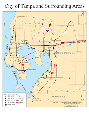
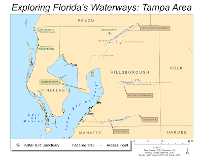
Here are the two maps from the ESRI exercises:




Learning ArcGIS Spatial Analyst

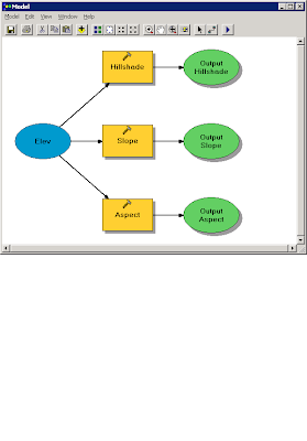
The first part of the ESRI Spatial Analyst Tools course focused on process models. The following image is the process model created for the exercise:

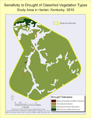
The second part focused on reclassifying data. The map below shows the vegetation layer reclassified and masked to show new classifications based on drought tolerance within a predefined study area:



The last map was created from the ArcGIS 3D Analyst module:



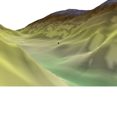
I actually went through, finished the module and passed the exam. I wanted to make a video but was not sure how to do it so just decided to post this image. I was not sure how to get the image though but found that you could post it to the clipboard which is what I did and then posted the clipboard to the Paint program to save it as a PNG file. I hope to go back and play with the Fly features some time in the future.

Week 9 - Vector Analysis II

The posted map was completed for the Week 9 Lab for the University of West Florida Online GIS Certification program class, Introduction to Geographic Information Systems (GIS 4043/L). The map was created using the ArcGIS ArcMap program.




This was a fun lab. I learned a lot and was challenged to think through the steps to get what was needed. I enjoyed this one quite a bit.

Lab Questions

Q1: Which tool was used: I used the Identity tool because it combines portions of features that overlap. The end results gave me the exact same set of overlay features as the Union overlay (I laid them on top of each other to verify). However, the intermediate step when the overlay was applied looked quite different as several areas were "missing". This makes sense when you look at the graphical depictions and read the overlay descriptions in the lab because Union combines features from both layers but Identity only combines portions of features that overlap. In this case because the road was my input feature the overlay created essentially matches the road buffer such that when over-layed on the original Union overlay you can see the discrepancies (See image below).



Off course now that I went to all this trouble I realize that I could have probably just used the Intersect Overlay and saved myself a step (and I thought I was being clever).

Q2 Which tool to exclude conservation areas: The Erase tool was used to exclude conservation areas because it excludes areas in the erase feature, here the conservation_area layer, that overlap the input feature or in our case the buffers_union layer.

Q3 How many features were in the possible sites layer: There were 79 features in the layer, the largest had an area of 7,765,034.49 Sq. Meters (7.7 Sq Km) and the smallest was 748.11 Sq. Meters.

Spring Break Fun!

The posted map was completed as an optional exercise during Spring Break the University of West Florida Online GIS Certification program class, Introduction to Geographic Information Systems (GIS 4043/L). The map was created use ArcGIS based on recent data downloaded from the State of Florida Department of Revenue.



The goal of the exercise was to take a ArcGIS shapefile of land parcels for Gulf County, Florida and join the parcel data to associated Tax Roll Data that was compiled as a table into a Comma Separated Value (CSV) file then use the information and the ArcGIS functions to determine the top four landholders in the county.

The instructions for the exercise were straightforward as was using ArcGIS to compile and analyze the information to obtain the desired result, a testament to the power and utility of a GIS system, particularly when the sources exist to provide the desired information. As someone with a lot of database and file conversion experience, I was very comfortable using the tools that are available in ArcMap much to my delight. I actually spent more time trying to compose a visually interesting map that displays the data in an easily identifiable way. Hopefully the final map outputed here does so.

Week 7 Data Editing in ArcGIS

The posted map was completed for the Week 7 Lab for the University of West Florida Online GIS Certification program class, Introduction to Geographic Information Systems (GIS 4043/L). The map is the same as was posted for the Week 6 Lab but several features have either been edited or added to the vector shapefiles on the map including adding a new feature shapefile for Athletic fields.



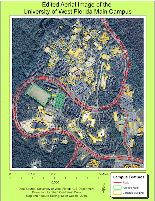
The lab was pretty straight-forward and required following the steps learned in the previous part of the lab as part of the ESRI Learning ArcGIS class. The only tip I could offer is to be patient while digitizing and do not be afraid to delete and start over.

Week 6 - Georeferencing Assignment

The posted map was completed for the Week 6 Lab for the University of West Florida Online GIS Certification program class, Introduction to Geographic Information Systems (GIS 4043/L). The map used an image registration process called georeferencing to link 2 seperate aerial images of the north and south sections of the campus to the overlaid vector layers of buildings and roads.



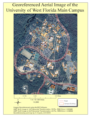
Having done some digitizing in the past I was a little familiar with the concept presented here but thought it was interesting to see how the images, especially the south section, moved after each point was referenced. The keys to being successful I thought were patience and the willingness to go back and re-evaluate all your previous points based on their Root Mean Square (RMS) value and image correctness after continuing to add points. Often I found that I could delete an old point whose RMS had gone up to ~7 or 8 and redo the point to an RMS of ~4 or 5 lowering the overall RMS total. I also found that it was important to try to place points on the road, provided it was relatively easy to select a location such as an intersection or crosswalk where you could be relatively close in your reference. Doing so seemed to be the best way to get the road image to line up with the road vector.

Week 5 - GIS Data Search Assignment

The posted maps were completed for the Week 5 Lab for the University of West Florida Online GIS Certification Program class, Introduction to Geographic Information Systems (GIS 4043/L).

The first map shows Hydrology and Man-made features of Indian River County, Florida including the county boundary, cities & towns, major roads, line and polygon hydrography and wetlands. Additionally, I have added DRG, DEM and DOQQ raster datasets to 3 adjacent quads across the middle of the county. I learned quite a bit making the map but spent way too much time on it. In particular I was not happy with the way some of the downloaded files attribute tables classified information and wanted to make my own but could not figure out how to add a text field to the attribute table and then fill it in, something I hope to learn soon. I was lucky with the shape of the county as it lent itself to leaving open areas for legends and such. I left my Florida layer turned on because it adds some extra contrast to the legends. All my shape files came from the Florida Geographic Data Library for this map and the next one. All were in the Alber's Conic projection.

The raster files came from the Land Boundary Information System (LABINS) and I attempted to re-project each of the layers to the Alber's projection which prove to be highly difficult and fraught with confusing results that may not be 100% successful. The DOQQ maps were the easiest because they were already in Alber's projections with matching False Easting and other information. By far the most difficult was the DRG because I could not seem to get the un-collared file to re-project properly.



Okay, this one is a little much, but I'm giving myself an E or A for Effort. I spent way too much time trying to work the elements of the map into a presentable theme and I'm not sure I was 100% successful. I probably should have provided less detail but even though it's a busy map, I do think everything is well organized and understandable, especially at the blow-up size. So in the end I'm satisfied with it. Basically I was focusing on the public lands and tried to categorize them in a meaningful way. The attribute table had three fields that seemed reasonable - Owner, Managing_A (Association?) and ManageInst (Managing Institute) which is the one I chose though i renamed it in the legend. I thought who managed each public land was an important piece of info to display. I created my own symbols for the invasive species which was one of the coolest things I learned on the assignment, also learned how to add transparency to a layer. In the invasive species attribute table were about 14 actual species but only the four listed by name were given a separate symbol because they had more then a few occurrences. I wanted to combine two fields, Common Name and Scientific Name, into one description for the legend but forgot how to do it. If I have time (unlikely) I may try to figure that out. At the last moment I added the Archie Carr NWR inset because that was where there was a large concentration of invasive species and since that was one of the map themes I thought it was needed.

The bottom line was I learned quite a bit about ArcGIS on this exercise.